Fully exempt pages have
FOI 3858 -
been deleted from the
Document 1
document set
s 22
From:
s 22
Sent:
Tuesday, 14 March 2023 11:10 AM
To:
s 22
Subject:
FW: A dynamic demand model for tobacco [SEC=OFFICIAL]
OFFICIAL
OFFICIAL
From: s 22
@TREASURY.GOV.AU>
Sent: Tuesday, 17 November 2020 10:16 AM
To: Kennedy, Darren <xxxxxx.xxxxxxx@xxxxxxxx.xxx.xx>
Cc: s 22
@TREASURY.GOV.AU>; s 22
@TREASURY.GOV.AU>;
s 22
@TREASURY.GOV.AU>; s 22
@TREASURY.GOV.AU>; s 22
@TREASURY.GOV.AU>
Subject: RE: A dynamic demand model for tobacco [SEC=OFFICIAL]
OFFICIAL
Hi Darren
Theta is in the final equation. I skipped some transformation steps in the middle. Please find them below.
The theoretical model (combining (1)+(2)) is
𝑣 = 𝑘 ( )
𝑌
(𝑣
)
𝜀 , (3)
Taking logarithms on both sides of (3), we have
ln(𝑣 ) = 𝜃ln (𝑘 ) + 𝑘 𝜃 ln(𝑝 ) + 𝑘 𝜃 ln(𝑦 ) + (1 − 𝜃) ln(𝑣
) + 𝜃ln (𝜀 ), (4)
Where 𝑝 =
If you compare (4) with the final equation we estimate,
ln(𝑣 ) = 𝛽 + 𝛽 ln(𝑝 ) + 𝛽 ln(𝑦 ) + 𝛽 ln(𝑣
) + 𝜀
𝛽 = 𝜃ln (𝑘 )
𝛽 = 𝑘 𝜃
𝛽 = 𝑘 𝜃
𝛽 = 1 − 𝜃
So theta is in the final equation and it is part of all the coefficients that we estimate. As shown above, the
adjustment affects both price and income elasticities of tobacco demand. The advantage of our model is it captures
these dynamics and provides an accurate estimation of the elasticities.
Please let me know if you have other questions and happy to discuss.
Kind regards,
s 22
OFFICIAL
1
From: Kennedy, Darren <xxxxxx.xxxxxxx@xxxxxxxx.xxx.xx>
Sent: Friday, 13 November 2020 6:19 PM
To: s 22
@TREASURY.GOV.AU>
Cc: s 22
@TREASURY.GOV.AU>; s 22
@TREASURY.GOV.AU>;
s 22
@TREASURY.GOV.AU>; s 22
@TREASURY.GOV.AU>; s 22
@TREASURY.GOV.AU>
Subject: Re: A dynamic demand model for tobacco [SEC=OFFICIAL]
Nicely explained s 22 thanks
I note that theta doesn’t make it into the final equation - I assume you use the estimate from the Breunig paper?
Darren
Darren Kennedy
Principal Adviser, Tax Analysis Division
The Treasury, Langton Crescent, Parkes ACT 2600
Phone +61 2 6263 3737
On 13 Nov 2020, at 5:18 pm, s 22
@treasury.gov.au> wrote:
OFFICIAL
Hi Darren
As requested, here is an outline of the dynamic demand model for tobacco we use for estimating
elasticity. The model is based on Bob Breunig and Carol Gisz’ (2008) paper especially the standard
approach part of the paper (attached).
The desired demand for tobacco consumption,vt* , can be modelled as
vt*=κ 1(PcP)tκ 2ytκ 3, (1)
wherePcP is the relative price - the ratio of tobacco pricePc to overall price for household
consumable goodsP; Y is real income or household disposable income divided by CPI;κ 2 is the price
elasticity of demand for tobacco that we need to estimate.
An important aspect of smokers’ behaviour pattern is they do not adjust how much they smoke
immediately after price changes due to habit and addiction. There are lags so we use the following
specification to capture the adjustment process (e.g. habit change). The harder the habit can change
(quitting or reducing the amount of tobacco smoked) the smallerθ is.
vt=(vt*)θ(vt-1)1-θ, (2)
θ=1, vt=vt* (full adjustment) θ=0, vt=vt-1(zero adjustment)
Ifθ=1, i.e. full adjustment, actual consumption is equal to the desired consumption
If θ=0, i.e. zero adjustment, actual consumption is equal to the last period actual consumption.
Combing (1) and (2) and taking logarithms, we have a dynamic model which we then estimate using
a dataset covering 40 years (1980-2020).
lnvt=β 0+β plnpt+β ylnyt+β vlnvt-1+εt
2
By definition, elasticity is percentage change in demand for one percentage increase in prices.β p is
the price elasticity.
After testing time series properties for each series, we have selected ARIMA (autoregressive
integrated moving average) to do the estimation.
Thanks s 22 for QAing the model and s 22 and s 22 for valuable comments/suggestions.
Please let me know if you have questions or comments on the model and happy to discuss the
above, estimation process and results anytime.
Kind regards,
s 22
Indirect Tax Modelling Unit | Tax Analysis Division | Revenue Group
Phone: s 22
| Mobile: s 22
The Treasury, Langton Crescent, Parkes ACT 2600
www.treasury.gov.au
Follow us: Twitter | LinkedIn | Facebook
Current work arrangements: I am working remotely Monday, Tuesday, Wednesday, and Friday.
OFFICIAL
<Breunig_Gisz.pdf>
OFFICIAL
3
FOI 3858 -
Document 2
s 22
From:
s 22
Sent:
Tuesday, 14 November 2023 2:20 PM
To:
s 22
; s 22
@ato.gov.au
Cc:
s 47E(d)
; s 22
Subject:
Tobacco: Forecasting, costing, & tax-gap methodology [SEC=OFFICIAL:Sensitive]
Attachments:
ITTSAB 2023-020_Tobacco excise_HL_1 Sept 2023 start date.pdf
OFFICIAL:Sensitive
Hi s 22
and s 22
Thanks for the chat yesterday. s 47E(d)
In relation to our tobacco forecasts, we firstly estimate the number of sticks and loose (kgs), which is based on
previous clearances and grown by Treasury’s internal tobacco consumption parameter (this is a base plus growth
modelling approach). We then multiply the clearances by the excise rate for each stick/kg, which is indexed to
AWOTE. AWOTE is grown over the forward estimates period by Treasury’s internal AWOTE parameter and, as
legislated, the indexation factor is worked out by dividing the most recent AWOTE amount by the highest AWOTE
amount for a previous June or December quarter that does not precede the December quarter 2012. Indexation is
applied every March and September. As with other heads of revenue, Treasury consults with Home Affairs and/or
the ATO in the course of developing the forecasts.
s 47E(d)
The model we use for tobacco
excise costings is in R, and as discussed, is quite complicated. In summary, it reads in clearances for sticks and loose
tobacco, AWOTE and excise rates from the forecasting model, prices, and policy adjustments. It then generates
excise rates for baseline and policy settings, for both sticks and loose tobacco. The model then generates a price
series to estimate the impact on tobacco demand as a result of the price increase. A point in time price for sticks and
loose is estimated from a sample of brands and a price series is generated (this is based on excise increases and also
now growth in the non-tax component of tobacco products). It then generates clearances based on price changes
(this is where the elasticity of -0.5% is applied). Estimates of revenue are then simply:
• Baseline revenue = baseline clearances*baseline rates
• Policy revenue = policy clearances*policy rates
s 47E(d)
1

s 47E(d)
Hope this helps and feel free to reach out if you have any questions. s 22
Thank you.
Kind regards,
________
s 22
Consumption Tax Unit, Indirect Tax and Tax System Analysis Branch
Tax Analysis Division
P +s 22
The Treasury acknowledges the traditional owners of country throughout Australia, and their continuing connection to land,
water and community. We pay our respects to them and their cultures and to elders both past and present.
s 22
OFFICIAL:Sensitive
2

FOI 3858 -
Document 3
s 22
From:
s 22
Sent:
Wednesday, 22 March 2023 10:34 AM
To:
Di Marco, Katrina; Kennedy, Darren
Cc:
s 47E(d)
; s 22
Subject:
RE: Update: Modelling tobacco elasticity [SEC=OFFICIAL:Sensitive]
OFFICIAL:Sensitive
Hi Kat and Darren,
Just circling back on this to confirm where we landed and provide further information on the descriptive statistics.
In our catch up last week we agreed to use the straight linear regression value from 2020, (which was -0.42),
however, the value for 2020 when using the updated underlying National Accounts data is -0.43. Apologies for not
thinking to provide this as an option prior to our meeting! Using the 2020 output to exclude COVID impacts, but with
updated data, seems the most sensible option and is the elasticity assumption we have used in our latest tobacco
costings provided to the TO.
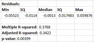
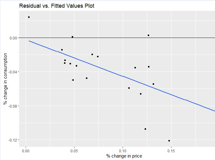
In relation to the R Squared values and residuals for the linear regression model (for the -0.43 elasticity), please see
the fol owing outputs:
1

Overall, the variability in the residuals indicate a fairly loose fit, and the R-squared values indicate that only around
34-38% of the variability in consumption can be attributed to price changes, however, the significant P value is at
least confirming that the relationship between change in consumption relative to change in price is statistically
significant. The straight linear regression may include years where consumption remains high (or higher), relative to
a price hike in a given year due to the delayed impact on smoker behaviour, which will reduce (or have a negative
impact on) the relationship between price and consumption.
The behavioural analysis from 2020 is a dynamic model using autoregression, therefore the descriptive statistics will
not be directly comparable to those for the linear regression model we are currently using. However, the chi
squared value from the 2020 behavioural approach in Stata was highly significant at 0.0001. This indicates that the
‘true’ relationship between prices and consumption is non-linear, because the lagged value as created in the
dynamic model is a better overall fit.
The output elasticity values for each 20 year regression also aren’t overly stable year to year, in that there can be
deviations of almost 0.1 per cent between years, however, all outputs from the mid-1990s onwards are consistently
around or between the -0.3 to -0.5 value, which is consistent with the literature. Our output of -0.43 is also in line
with the current literature on tobacco elasticities for other high-income countries are generally around -0.4 to -0.44.
It is also not substantially different from that produced by the 2020 behavioural approach (-0.414), therefore it is a
‘safe’ assumption to use at this time.
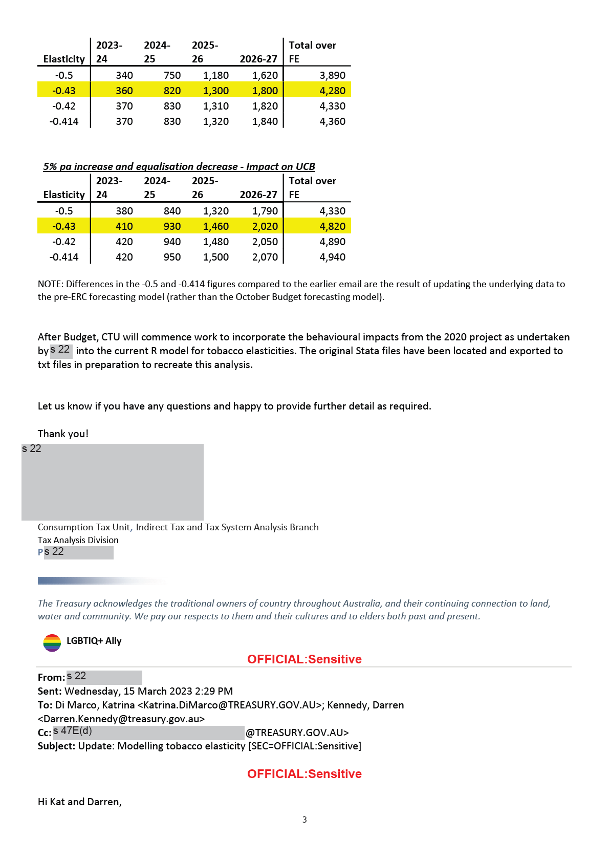
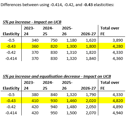
Differences between using -0.414, -0.42, and -0.43 elasticities:
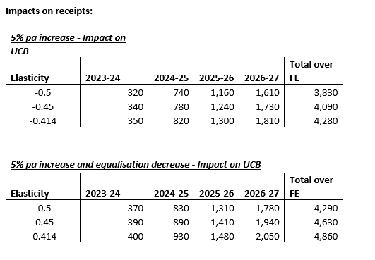
5% pa increase - Impact on UCB
2

As you are aware, we have been looking into an appropriate elasticity assumption for tobacco. Previously an
elasticity assumption of -0.5 was used as it was published in a 2019 Treasury paper on tobacco model ing by John
Clark. We have identified that -0.5 is slightly higher than what is found in the literature and also what our model ing
shows using several different methodologies (-0.414 to -0.45). We would like your input as to which elasticity
assumption you are comfortable with for us to use for this costing.
Al model estimates are consistent with the literature, which general y suggests an elasticity in the range of -0.25 to -
0.5 for high-income countries, with many at around -0.4.
We recommend an elasticity of -0.414, which was agreed by Darren and Gil ian in 2020 and incorporates habitual
behavioural impacts from smoking and is not affected by COVID.
Elasticity options are as fol ows:
- -0.5 is the current elasticity assumption which is based on straight linear regression model ing and published
in the 2019 Treasury paper.
- -0.414 is the elasticity that incorporates the habitual behavioural impacts as modelled in 2020
o Does not include most recent National Accounts data (from 2020 to 2022 - but these years are
COVID affected anyway)
- -0.42 is the updated elasticity based straight linear regression (only on change in consumption relative to
changes in prices) for 2020
o Does not include the most recent National Accounts data (from 2020 to 2022 - COVID affected
anyway)
- -0.45 is the elasticity based only on change in consumption relative to changes in prices and updated for
2023
o Uses updated National Accounts data for 2022, but takes a 10 year average to smooth out policy
impacts and COVID induced volatility
Impacts on receipts:
5% pa increase - Impact on
UCB
Total over
Elasticity
2023-24
2024-25 2025-26 2026-27 FE
-0.5
320
740
1,160
1,610
3,830
-0.45
340
780
1,240
1,730
4,090
-0.414
350
820
1,300
1,810
4,280
5% pa increase and equalisation decrease - Impact on UCB
Total over
Elasticity
2023-24
2024-25 2025-26 2026-27 FE
-0.5
370
830
1,310
1,780
4,290
-0.45
390
890
1,410
1,940
4,630
-0.414
400
930
1,480
2,050
4,860
Further context
Modelling the impacts of habit and addition:
- As part of a project in 2020, econometric model ing was done to account for the habitual nature of smoking
and the potential for price changes to have a delayed impact on behaviour (based on Breunig’s work on
fuels).
4

- Smokers do not adjust how much they smoke immediately after price changes due to habit and addiction
and as part of the tobacco elasticities update project in 2020,s 22 used econometric modelling to account
for the potential for price changes to have a delayed impact on behaviour. The new approach includes lags to
account for behaviour change (basically the harder it is to quit or reduce the amount of tobacco smoked, the
smaller the equivalent econometric value is).
- This produced an elasticity of -0.414
- This work was presented and agreed by Darren and Gillian at the time as the elasticity assumption to use
from then on
- This work was done in Stata and not transferred to the R model
- With no further policy changes relating to tobacco, this new elasticity was not entered into TOBIAS
- Time does not allow us to add this into the straight linear regression model for elasticities in R for this
costing, which means 2020 is the most recent year used for any underlying National Accounts data
General:
- Our modelling and the literature indicate that overall elasticities don’t tend to change over time (see chart
below)
- Elasticities do differ across demographic cohorts (ie. young people and those on a low income are more price
sensitive)
- In Australia, prevalence of smoking is higher in: low SES, remote and aboriginal communities, as well as older
people and those with poor mental health (AIHW)
o Australia already has some of the lowest smoking rates in the world, following a steady decline since
the early 1990s.
o We also have the most expensive cigarettes in the OECD (OECD, 2022)
o Increases in tobacco excise will be largely regressive
Elasticities output - Change in consumption relative to change in price (additional behavioural impacts not
included) - Model updates to 2023:
Currently, neither modelling approach will account for:
- Impacts of the policy changes (ie. hoarding and stockpiling before policy start dates, and further reduced
consumption over time as a result of the policy)
- Short-term versus long-term policy impacts
- Types of elasticities (ie. insider vs outsider – whether people quit or scale back but keep smoking, or do
fewer people start smoking)
- Substitution effects (whether people may switch to vaping and/or the impacts of the black economy)
- Demographics of smokers in Australia and their varying elasticities (younger people have higher elasticities
than older people, lower income smokers have higher elasticities than higher income smokers)
5

- When time allows, further work could be done to account for these factors/some of these factors in the
model, but currently both time and data is limited (ie. No HES since 2015-16, and the NHS in 2021 was a
break in timeseries – done online and during COVID).
Kind regards,
________
s 22
Consumption Tax Unit, Indirect Tax and Tax System Analysis Branch
Tax Analysis Division
P s 22
The Treasury acknowledges the traditional owners of country throughout Australia, and their continuing connection to land,
water and community. We pay our respects to them and their cultures and to elders both past and present.
s 22
OFFICIAL:Sensitive
6

FOI 3858 -
Document 5
Tobacco Elasticities Model: Linear versus lagged regression
October 2023
Background
Treasury’s approach to tobacco elasticity is published in the Treasury Working Pater, ‘Tobacco Excise:
Historical trends and forecasting methodology’, June 2019, by Jonathan O’Bannon and John Clark.
This approach is based on a linear regression model which analyses the change in consumption relative to
the change in price. In 2020 this model was developed in R to facilitate its use in future costings. At this time,
additional econometric analysis to incorporate lagged behavioural responses to price and income changes
using a dynamic regression was undertaken in Stata. The results were presented within Treasury and agreed
as a more accurate approach, however the project wrapped up before it could be transferred into R to
facilitate future use.
23-24 Budget Costing: Tobacco excise increase elasticity options
In the lead up to 23-24 Budget the government proposed changes to the tobacco excise system. Elasticities
had not been revisited since 2020, so the following options were investigated:
-
The standard linear regression approach based on O’Bannon and Clark’s method but using
updated underlying National Accounts data. This provided an output of:
o -0.46 for 2022 (including the COVID affected)
o -0.45 for 2022 if taking a 10 year average to smooth out policy and COVID impacts
o -0.43 for 2020 (excluding the COVID affected years).
o -0.42 for 2020 if underlying National Accounts data was not updated
-
The dynamic regression output from Stata based on 2020 data, which provided an output -0.414
-
The published elasticity of -0.5 based on the Working Paper.
The following tables (supplied to SES in March 2023) show the impact of different elasticities on two costing
options:

Tobacco Elasticities Model: Linear versus lagged regression
October 2023
Differences comparing -0.5, -0.45, and -0.414 elasticity options:
Decision to use -0.5
After all options and impacts on revenue were considered, the published elasticity of -0.5 was selected as
the most appropriate option for this costing. The other options were thought to be a bit low, which caused
concerns regarding potential over-estimation of any expected revenue. In addition, the dynamic regression
approach was based on earlier 2020 output from Stata, and as the model was not in R, it could not be easily
updated for comparison and validation. As a result, the published figure of -0.5 was considered as the most
defensible option given the scrutiny this costing may likely attract.
Post 23-24 Budget: Recreating the dynamic regression in R
Dynamic regression is considered by internal Treasury econometrists as the most accurate way to estimate
tobacco elasticity. It accounts for the impact of both price AND income changes and also accounts for the
‘stickiness’ or addictiveness of smoker behaviour in response to price increases. This improves the accuracy
of estimated revenue implications of proposed changes in the tobacco excise system.
Original testing indicated that consumption lags behind any changes in price and income by around a year,
meaning that it takes a year or so before changes in either price or income affect actual behaviour, in either
direction. For example, if income goes up, it takes a year or so before consumption increases, and if price
goes up, it takes a year or so for consumption to decrease.
Following the 23-24 Budget, the dynamic regression model was recreated in R and tested against both the
original data from Stata, and the original linear regression approach.
In short, testing and QA processes demonstrated that the R model is accurately recreating the dynamic
regression which was in Stata, and that this model provides a more accurate estimation of the impact of
both price and income on the consumption of tobacco compared to the linear regression.

Tobacco Elasticities Model: Linear versus lagged regression
October 2023
Regressions were conducted based on 20, 25 and 40-year samples, and the most stable output was based on
a 40-year dynamic regression. All initial testing was undertaken on 2020 data to most closely recreate the
original work in Stata. The Stata output from 2020 was based on a 40-year regression, with an output value
of -0.414. The corresponding R output using 2020 data had an output of -0.433. See notes on
methodology/validation for explanation.
Using updated underlying data to March 2022,
the new proposed elasticity is -0.44. This is the output for
2020 based on a 40 year regression. Elasticity outputs for 2021 and 2022 appear to be impacted by COVID so
recommend using the output for 2020.
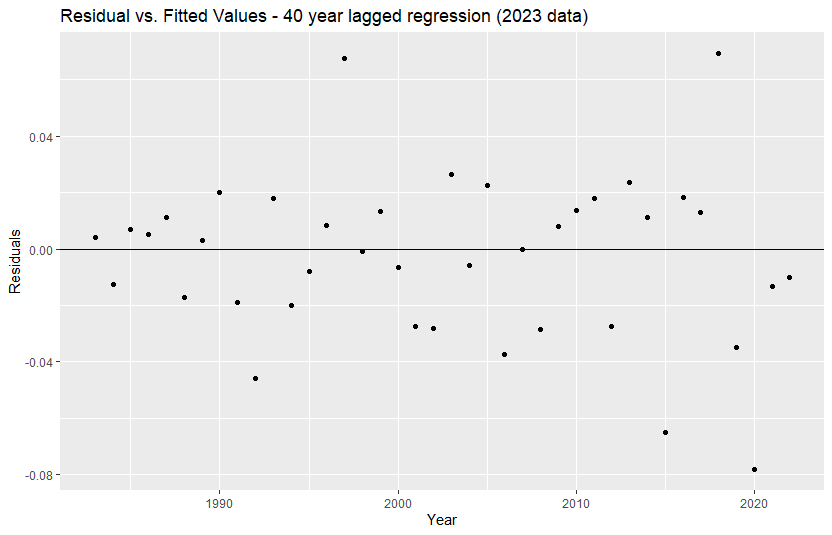
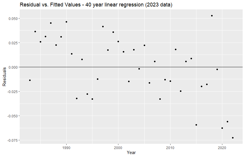
Charts 1 and 2 show the residuals from the lagged regression and the linear regression. The lagged
regression is a better fit as the residuals are generally more evenly spaced and lack any clear trends, whereas
a trend is evident in the linear regression. This shows that the linear regression model Is not the best fit for
the data.
Chart 1: Residual values: 40-year lagged regression
Chart 2: Residual values: 40-year linear regression


Tobacco Elasticities Model: Linear versus lagged regression
October 2023
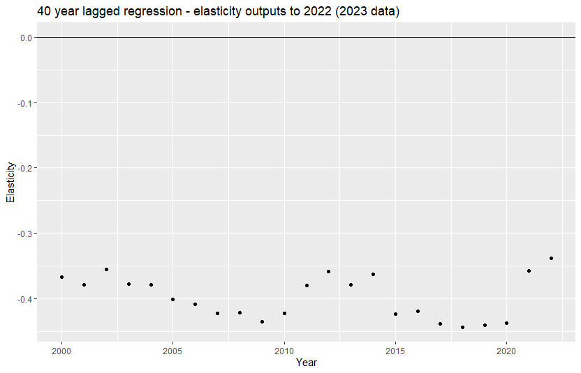
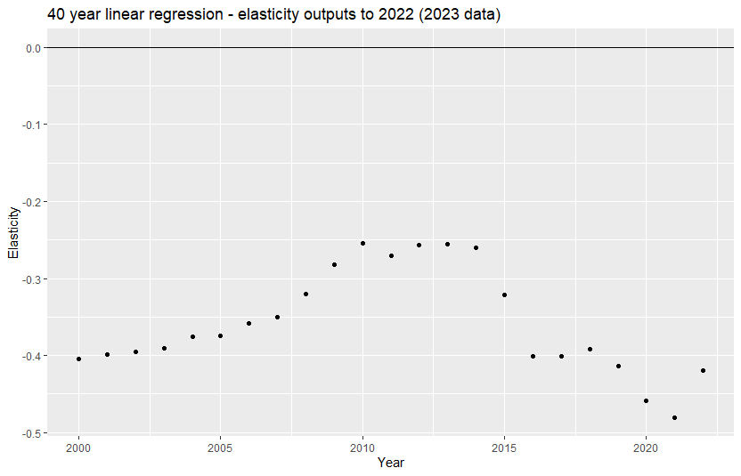
Charts 3 and 4 show the elasticity outputs for the 40 years to 2022 for the lagged regression and the linear
regression respectively. The lagged regression provides more stable outputs, meaning that there is less
volatility in the outputs over time compared to the linear regression. However, note the more volatile
outputs in COVID-affected years (2021 and 2022).
Chart 3: Elasticity outputs over time for the 40-year lagged regression

Tobacco Elasticities Model: Linear versus lagged regression
October 2023
Chart 4. Elasticity outputs over time for the 40-year linear regression
Post 23-24 Budget: The way forward
1. Agree to changed tobacco elasticity methodology (and output of -0.44?).
2. After a costing request is received, update the underlying National Accounts data in the Tobacco
Elasticities Model which is now the 40-year dynamic regression model.
3. Consider which output is the most appropriate given market forces, policy context, and the COVID
affected years of 2021 and 2022.
4. Sense-check the output and liaise with SES before using the output in TOBIAS as there are broader
factors and sensitivities to consider when undertaking a tobacco costing (ie. policy impacts,
government priorities, industry information).
Future improvements
One way to improve the elasticity assumption in the future will be to incorporate vaping as an additional
variable, if and when an HFCE series for vaping products becomes available. This is based on the assumption
that there is substitution occurring between smoking and vaping, in either direction, depending on the price
of one relative to the other.
Notes on validation:
Underlying algorithms for the arima model are different in R and Stata, which may explain the differences
we are seeing when recreating the 2020 figures based on same data as Ying’s earlier model (0.433 in R
versus 0.414 Stata).
Tobacco Elasticities Model: Linear versus lagged regression
October 2023
The underlying arima model equation (forecast package) was checked by TAD analyst s 22
. It was
confirmed the arima model is accurately recreating the underlying theoretical model detailed by s 22
in
her original presentation and as created in Stata:
ln(𝑣𝑡) = 𝛽 + 𝛽 ln(𝑝
ln(𝑦
ln(𝑣
0
𝑝
𝑡) + 𝛽 𝑦
𝑡) + 𝛽 𝑣
𝑡−1) + 𝜀𝑡,
The values for the arima model are as follows:
Autoregressive term of 1 (meaning the dependent variable, consumption, lags by one year compared to
income and price), differencing of 2 for each time series variable for it to be stationary, and no cointegration.
P = 1, D = 2, Q = 0
Regardless of whether the forecast, stats, TSA or fable packages were used, arima (all lower case) takes the
consumption time series (which is lagged by one year) and analyses the impacts of two exogenous variables:
price and income. Testing on all packages in R provided the same results.
Arima (with a capital A) seems to combine the external regressors and only provides one coefficient, but
there would be a way to make it output the same value. The underlying equation is doing the same thing as
the arima. This is the same as the ARIMA (all caps). It required slightly different inputs compared to the
arima, but theoretically should be doing the same thing.
Testing was also undertaken using the arimax function in the in TSA package. This produced the same results
as the original arima (and it was confirmed it is the same function as arima in the TSA package)
We tried to recreate ARMAX in sysid package but encountered difficulties. The ARMAX function requires
different ‘ordering’ values, and also does not use p d q values like the arima. ARMAX also requires stationary
data but does not do any differencing, therefore this data is not appropriate for an ARMAX model.
Testing of lagged consumption time series only (with external regressors removed) also demonstrated the
external regressors are ‘working’ on consumption as the results varied significantly without them.
95% Confidence Intervals also indicate the acceptable variability, and our results are well within range
considering the different algorithms between R and Stata.
After final testing, a warning on the summary function popped up which wasn’t there previously.
Investigated to the extent possible but not a lot of information on it. Coefficient output was the same.


